
What a graph database is and how AI agents use it
In the previous article we showed how a vector database finds semantically similar text. But for the question “which of our customers use a technology managed by the team of the person who left last month?” similarity is useless — the answer doesn’t go through similar words but through a chain of relationships. Graph databases exist precisely for such questions. We’ll go in depth into how they work (property graph, Cypher, index-free adjacency), when they make sense instead of a relational database and SQL or a vector database — and then three ways AI agents use them today: text2Cypher, GraphRAG and temporal graph memory.
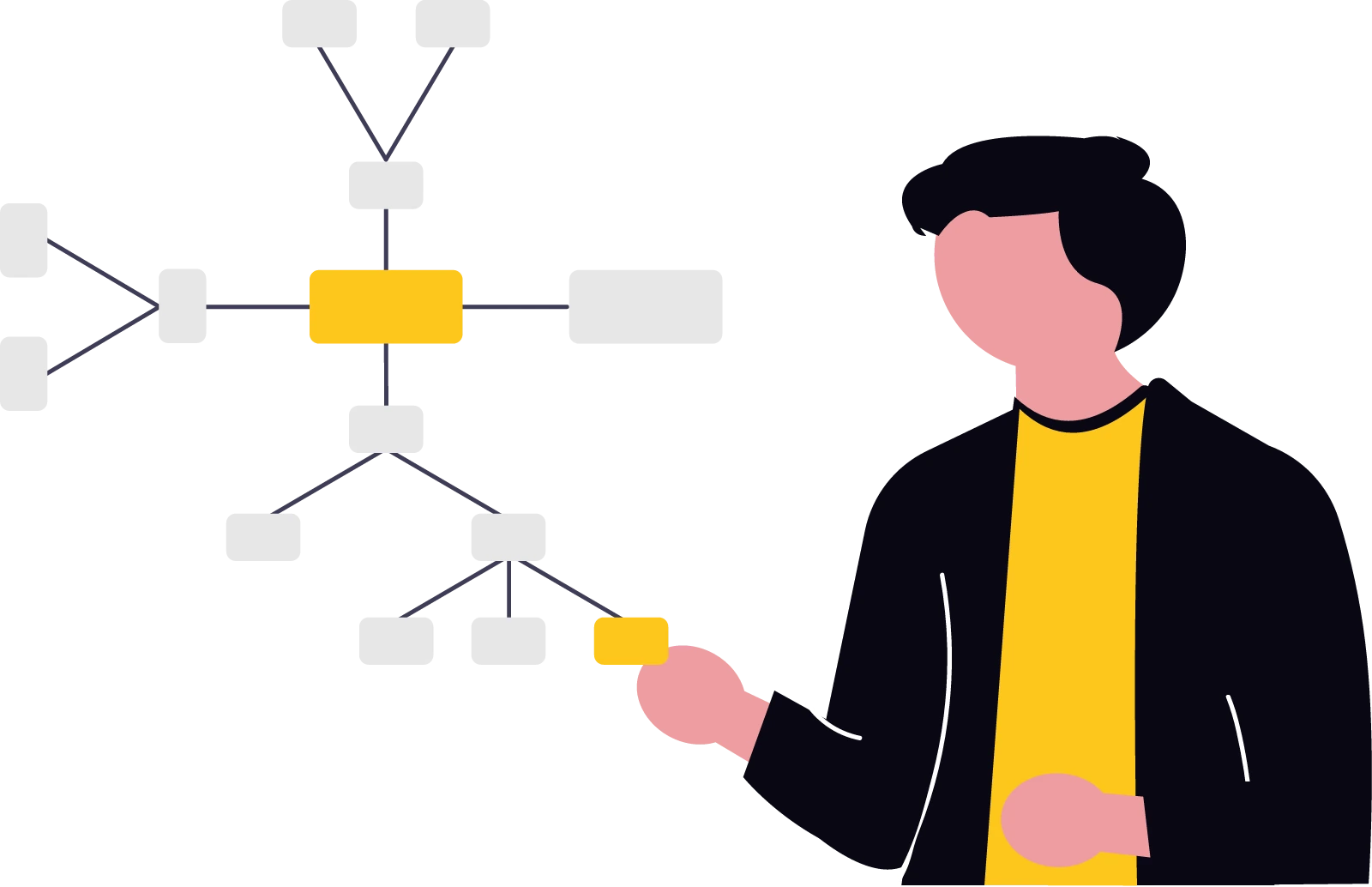
In one sentence
A graph database makes sense the moment the answer lies neither in a single record nor in similar text, but in a path across several relationships: who is related to whom, through what and with what impact.
Relationships as first-class data
Relational databases have always handled relationships — they’re named after them. But in them a relationship is derived: it exists only as a match of foreign key values that the database has to recompute with a JOIN on every query. For one or two hops this works great. The problem arises when you ask in depth:
- Which colleagues of my colleagues know Kubernetes? (2 hops)
- Through whom do I know the CTO of company X? (unknown number of hops)
- Which components in the system will be affected if this service fails? (transitive dependencies)
- Orders, devices and IP addresses form a suspicious circle — fraud? (a cycle in the graph)
Every additional hop means another JOIN in SQL, intermediate results grow and the query planner sweats. For a query of unknown depth (“find a path”), SQL without recursive CTEs has no way to even ask the question — and with them a simple question quickly becomes a hard-to-read query. A graph database flips the perspective: the relationship is stored as a full-fledged record — a physical pointer between two nodes, with its type, direction and properties. Moving from a node to its neighbour is not a join but following a pointer.
Property graph: nodes, edges, properties
The most widespread model is the property graph (labeled property graph). It consists of four building blocks:
- Nodes — entities: people, companies, products, documents.
- Labels — the type of node (
:Osoba,:Firma); a node can have several. - Edges (relationships) — named, directed relationships between two nodes (
:PRACUJE_V,:OVLADA). - Properties — key-value data on nodes and edges: for the relationship “works at”, for example since when and in what position.

Alongside the property graph there is also the older academic model RDF (subject–predicate–object triples, queried via SPARQL), which you’ll meet in the semantic web and ontologies — e.g. Wikidata. In the practice of AI applications the property graph dominates today, among other reasons because in 2024 it got its own ISO standard GQL — the first new database language standard since SQL (1987).
Cypher: SQL for graphs
The most used query language is Cypher from Neo4j (and its open variant openCypher, on which the GQL standard is also based). Its charm is that a query looks like ASCII art of the graph: you write nodes in round brackets, relationships in square brackets with an arrow. The pattern from the diagram above:
// vytvoreni dat: MERGE = vytvor, pokud neexistuje
MERGE (anna:Osoba {jmeno: "Anna"})
MERGE (beeit:Firma {nazev: "Turing Institut"})
MERGE (k8s:Technologie {nazev: "Kubernetes"})
MERGE (anna)-[:PRACUJE_V {od: 2024, pozice: "devops"}]->(beeit)
MERGE (anna)-[:OVLADA]->(k8s)

// kdo v Turing Institut ovlada Kubernetes?
MATCH (o:Osoba)-[:PRACUJE_V]->(:Firma {nazev: "Turing Institut"}),
      (o)-[:OVLADA]->(:Technologie {nazev: "Kubernetes"})
RETURN o.jmeno
The real power shows in queries that would be torture in SQL. Variable path length is written with an asterisk, the shortest path has a built-in function:
// kolegove kolegu (presne 2 skoky po vztahu ZNA), bez prime znamosti
MATCH (ja:Osoba {jmeno: "Anna"})-[:ZNA*2]-(doporuceni:Osoba)
WHERE NOT (ja)-[:ZNA]-(doporuceni) AND doporuceni <> ja
RETURN DISTINCT doporuceni.jmeno

// pres koho se znam s CTO firmy X? (nejkratsi cesta, max 6 skoku)
MATCH cesta = shortestPath(
    (ja:Osoba {jmeno: "Anna"})-[:ZNA*..6]-(cto:Osoba {pozice: "CTO"})
)
RETURN [osoba IN nodes(cesta) | osoba.jmeno] AS retez

// dopad vypadku: vsechno, co primo ci neprimo zavisi na sluzbe
MATCH (s:Sluzba {nazev: "auth-api"})<-[:ZAVISI_NA*1..]-(zasazene)
RETURN DISTINCT zasazene.nazev
Why is it fast? The key property of native graph databases is called index-free adjacency: each node holds direct pointers to its edges, so a step to a neighbour is a constant-cost operation — independent of the database size. A relational JOIN has to look up neighbours in an index whose cost grows with the number of rows (and without an index it’s a scan). A traversal of a million-node graph to depth 4 thus visits only the explored neighbourhood, while a fourfold self-join of the relationship table touches whole indexes. The price is weaker support for bulk analytical queries across all the data — there the relational model and columnar databases still lead.
Three paradigms side by side
| Databases | What it answers | Typical question |
|---|---|---|
| Relational | structured facts and aggregations | “How many orders did we have in June by region?” |
| Vector | semantic similarity | “Find documents that talk about the same thing as this query.” |
| Graph | connections and paths between entities | “How are these two things related and through what?” |
They are not competitors but complements — and modern AI applications often combine all three. A graph database pays off when the relationships themselves carry the value: recommendations, fraud detection, dependency analysis, organisational knowledge, master data. It doesn’t pay off for storing flat records without connections — there the relational model is both simpler and faster.
Among specific products the biggest is Neo4j (native graph, Cypher, vector index in the core, free community edition), a fast in-memory alternative is Memgraph, a lightweight choice for embedded use is Kùzu (the graph counterpart of SQLite) and FalkorDB targets GraphRAG scenarios directly. In the cloud there are Amazon Neptune or Azure Cosmos DB (Gremlin API).
Knowledge graph: a bridge between text and graph
For an agent to walk a graph, the graph must first exist. With structured data (CRM, information systems) it’s a matter of import. More interesting is extraction from unstructured text: an LLM reads documents and pulls out entity – relationship – entity triples, from which a knowledge graph is built. This used to be a demanding NLP discipline; today it’s a single pass through a model with a suitable prompt — LangChain has a ready-made LLMGraphTransformer for it:
from langchain_experimental.graph_transformers import LLMGraphTransformer
from langchain_neo4j import Neo4jGraph
from langchain_openai import ChatOpenAI
from langchain_core.documents import Document

graph = Neo4jGraph(url="bolt://localhost:7687", username="neo4j", password="heslo")

transformer = LLMGraphTransformer(
    llm=ChatOpenAI(model="gpt-4.1", temperature=0),
    allowed_nodes=["Osoba", "Firma", "Technologie", "Projekt"],
    allowed_relationships=["PRACUJE_V", "OVLADA", "POUZIVA", "VEDE"],
)

dokumenty = [Document(page_content=
    "Anna vede projekt Phoenix pro klienta AlfaCorp. "
    "Projekt bezi na Kubernetes a Anna je zaroven devops inzenyrka Turing Institut.")]

grafove_dokumenty = transformer.convert_to_graph_documents(dokumenty)
graph.add_graph_documents(grafove_dokumenty)
# vysledek: (Anna)-[:VEDE]->(Phoenix), (Phoenix)-[:POUZIVA]->(Kubernetes),
#           (Anna)-[:PRACUJE_V]->(Turing Institut), ...
Restricting allowed_nodes and allowed_relationships is not a detail: without it the model invents different types for the same thing every time (ZAMESTNAN_U vs. PRACUJE_PRO) and the graph falls apart into unconnectable islands. We’ll come back to the pitfalls of extraction.
How agents use graphs
And now the main part. In the article on agents we described the loop in which an agent calls tools; with vector databases we saw the roles of knowledge base and memory. A graph database fits into this puzzle in three ways, which are often combined in practice.
Way 1: text2Cypher — the agent writes the queries itself
The most straightforward integration: give the agent a tool that translates a natural-language question into Cypher, runs it and returns the result. The LLM receives the graph schema (labels, relationship types, properties) and the question; the generated query is executed and the data travels back into the context. In LangChain it’s a ready-made component, GraphCypherQAChain:
from langchain.agents import create_agent
from langchain.tools import tool
from langchain_neo4j import GraphCypherQAChain, Neo4jGraph
from langchain_openai import ChatOpenAI

graph = Neo4jGraph(url="bolt://localhost:7687", username="neo4j", password="heslo")

cypher_chain = GraphCypherQAChain.from_llm(
    ChatOpenAI(model="gpt-4.1", temperature=0),
    graph=graph,
    allow_dangerous_requests=True,   # viz uskali nize!
)

@tool
def zeptej_se_grafu(otazka: str) -> str:
    """Odpovi na otazku o lidech, projektech a technologiich z firemniho grafu."""
    return cypher_chain.invoke({"query": otazka})["result"]

agent = create_agent(model="openai:gpt-4.1", tools=[zeptej_se_grafu])
Unlike vector RAG, the model receives precise structured facts, can aggregate (“how many projects does each team lead?”) and the answer is auditable — you can read and verify the generated Cypher. The weakness: quality stands and falls with knowledge of the schema and the model’s ability to write correct queries; text2Cypher trips over a crooked schema or exotic queries. That’s why in production it pays to add few-shot query examples and validation of the generated Cypher before execution.
Way 2: GraphRAG — retrieval along relationships
Vector RAG has two systemic blind spots. Multi-hop questions: the answer arises from combining facts from several documents that are not similar to each other (the document about Anna doesn’t mention AlfaCorp, the document about AlfaCorp doesn’t mention Anna — only the Phoenix project connects them). And global questions: “what are the main topics in these documents?” has no similar chunk that could be found — the answer requires a view of the whole.
GraphRAG from Microsoft Research solves both: during indexing it extracts a knowledge graph from the documents, divides it with the Leiden algorithm into hierarchical communities (thematic clusters of entities) and has an LLM summarise each community. At query time it then offers several strategies:
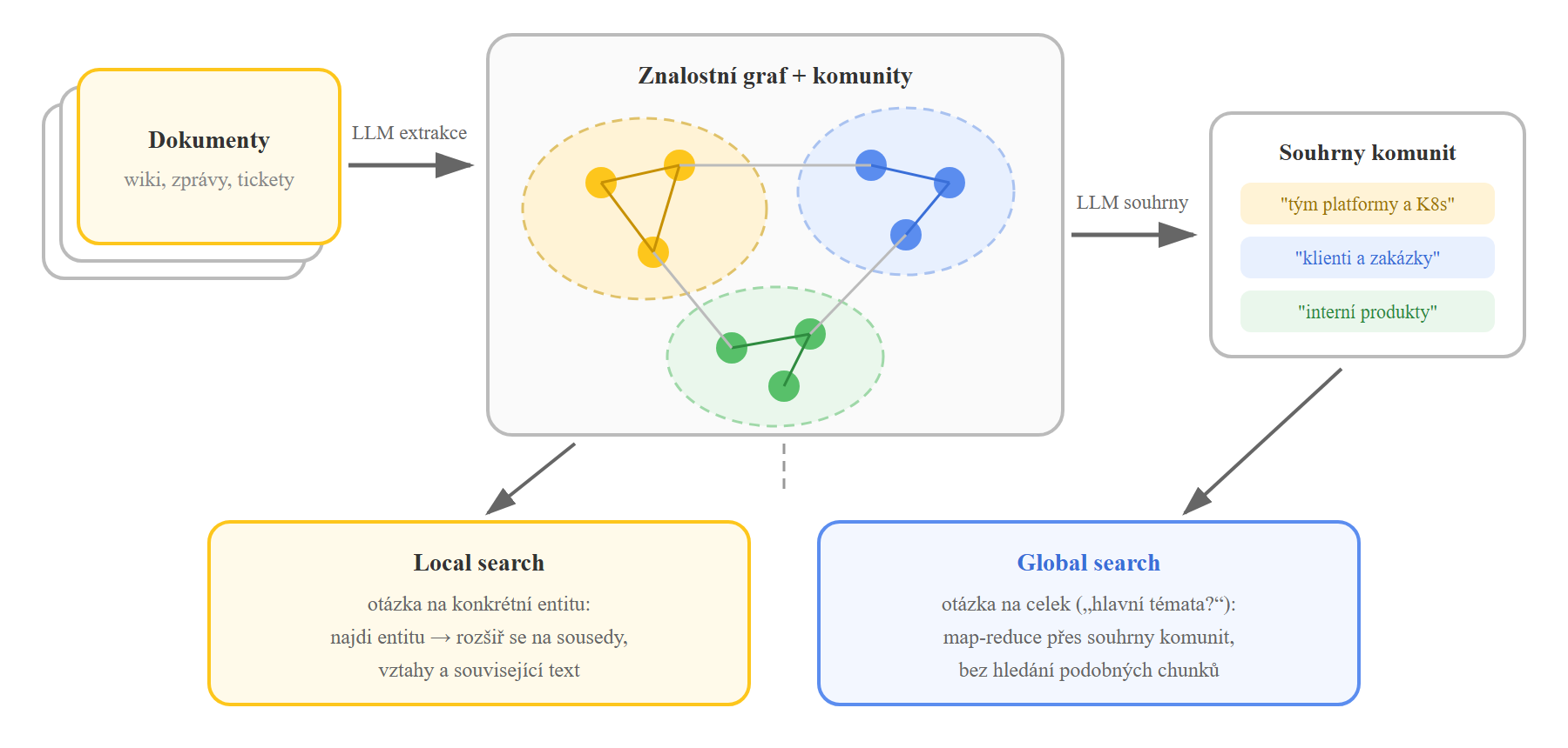
- Local search — for questions about specific entities: it finds the entry nodes (typically by vector search), expands along edges to neighbours, relationships and associated text chunks. This is exactly what solves multi-hop questions: the path Anna → Phoenix → AlfaCorp exists in the graph even though no single document contains it in full.
- Global search — for questions about the whole: map-reduce over community summaries, from which the LLM composes an answer about the topics and trends of the entire corpus.
- DRIFT search — a combination of both: it starts globally and iteratively drills down locally.
The price for all this: indexing means pushing the entire corpus through an LLM (extraction) and then once more (summaries), which for large collections costs real money and hours of time — and when data changes, the relevant part has to be recomputed. GraphRAG therefore makes sense for relatively stable knowledge corpora you query a lot; for rapidly changing data consider a lighter variant (local search only over a continuously updated graph) or the following approach.
Way 3: a temporal graph as agent memory
With vector memory we ran into the ageing problem: the agent confidently recalls last year’s truth. A vector store can’t do much about it — the two embeddings of the sentences “Anna works at AlfaCorp” and “Anna works at Turing Institut” are similar and both get returned. Graph memory has a more elegant solution: a fact is an edge with a validity period.
The pioneer is the open-source framework Graphiti (the core of the Zep memory platform, described in the paper Zep: A Temporal Knowledge Graph Architecture for Agent Memory). Each edge carries bi-temporal data: when the fact was valid in the real world (valid_at, invalid_at) and when the system learned about it (created_at, expired_at). When new information arrives in memory that contradicts an existing edge, the LLM recognises the conflict and invalidates the old edge — it sets its end of validity but doesn’t delete it:

The result: the agent can answer what is true now, what was true at any time in the past, and never mixes the two versions together. Moreover, the memory updates incrementally with every conversation (no hour-long reindexing as with GraphRAG) and retrieval combines semantic, full-text and graph search. Usage takes a few lines:
from graphiti_core import Graphiti

graphiti = Graphiti("bolt://localhost:7687", "neo4j", "heslo")

# po kazde konverzaci: uloz epizodu, extrakce a invalidace probehnou automaticky
await graphiti.add_episode(
    name="schuzka-2026-07-07",
    episode_body="Anna potvrdila, ze od kvetna vede devops tym v Turing Institut. "
                 "Projekt Phoenix pro AlfaCorp predala Petrovi.",
    reference_time=datetime(2026, 7, 7),
)

# pozdeji, v jine konverzaci: hybridni vyhledani relevantnich faktu
vysledky = await graphiti.search("kdo ted vede projekt Phoenix?")
for hrana in vysledky:
    print(hrana.fact)   # "Petr vede projekt Phoenix (od 2026-05)"
Graphs and vectors: not either–or
The attentive reader has noticed that the two technologies intertwine: GraphRAG finds entry entities by vector, Graphiti combines semantic and graph search, Neo4j has had a vector index directly in its core since version 5. The established pattern of modern AI applications is vector entry, graph expansion: the embedding finds relevant nodes (you don’t have to guess the exact name of the entity) and traversal along edges collects the connections similarity would never find. In Cypher this pattern looks like this:
// 1) vektorovym indexem najdi vstupni uzly
CALL db.index.vector.queryNodes('entity_embeddings', 5, $dotaz_embedding)
YIELD node AS entita, score

// 2) grafova expanze: posbirej okoli do hloubky 2
MATCH (entita)-[vztah*1..2]-(soused)
RETURN entita.nazev, score,
       collect(DISTINCT soused.nazev) AS souvislosti
ORDER BY score DESC
Pitfalls you’ll hit in practice
- Extraction quality decides everything. A knowledge graph is only as good as the triples it was built from. Restrict node and relationship types with a schema, deduplicate entities (“Turing Institut” vs. “Turing Institut s.r.o.” must be one node — so-called entity resolution) and evaluate the extraction manually on a sample.
- Text2Cypher is executing generated code. The LangChain parameter isn’t called
allow_dangerous_requestsby accident: the LLM can also generateDETACH DELETE. Connect the agent under a read-only account and validate queries, ideally with a whitelist of allowed constructs. - Cost and latency of LLM extraction. GraphRAG indexing of a large corpus costs tens to hundreds of dollars and hours; Graphiti in turn adds LLM calls to every episode. Account for this in the budget and for voluminous data consider a cheaper model for extraction and a more expensive one for answers.
- Modelling requires thought. A graph tempts you to make a node out of everything. A good rule: nodes are things you’ll ask about; properties are data you’ll filter by; edges are relationships you’ll walk along. If a query will never traverse an edge, it has no business in the graph.
- Evaluate retrieval, not impressions. Just as with vector RAG: a set of test questions with known answers and measurement of whether the graph returns the right facts. For multi-hop questions test the paths too (what the answer goes through), not just the final text.
What to do about it in practice
- Start with questions, not technology. If your questions sound like “find similar”, vectors suffice. As soon as they sound like “how are these related”, “through what” or “what happens if”, it’s time for a graph.
- To try it out: Neo4j in Docker (
docker run -p 7474:7474 -p 7687:7687 neo4j) and the web-based Neo4j Browser, where you see and click through the graph — with graphs, visualisation is half of understanding. For embedded experiments, Kùzu. - For RAG over a stable corpus consider GraphRAG (local + global search); for live agent memory a temporal graph (Graphiti). Don’t combine both right at the start — each has its own operational overhead.
- Put the graph schema into the agent’s prompt and keep it small and consistently named; every unnecessary relationship type degrades both text2Cypher and extraction.
- Combine with vectors: vector entry, graph expansion. And the order of results in the context is still subject to the U-curve — the most important facts at the edges.
Want agents with real memory?
In the AI Agent Developer course we build agents with tools, RAG and memory — from vector stores to knowledge graphs. You’ll find the broader context of LLMs and data pipelines in the Artificial Intelligence for Programmers, Science and Data Analytics course. And if you missed the previous part, read about vector databases, which this article follows on from.
Sources and further reading
- Edge et al.: From Local to Global: A Graph RAG Approach to Query-Focused Summarization (Microsoft Research, 2024) and the GraphRAG documentation
- Rasmussen et al.: Zep: A Temporal Knowledge Graph Architecture for Agent Memory (2025) and Graphiti on GitHub
- Neo4j Getting Started and Cypher Manual — official documentation
- LangChain Neo4j Integration — GraphCypherQAChain, LLMGraphTransformer, vector index
- ISO/IEC 39075:2024 GQL — the query language standard for property graphs
- Robinson, Webber, Eifrem: Graph Databases (O’Reilly) — index-free adjacency and modelling in depth
